
Preprint, version 1 (October 2026). Not peer reviewed. This is the author’s manuscript, prepared for submission to a peer-reviewed journal. Download: PDF · Word · reproducibility package (zip) · code on GitHub with code, results and the two independent audits.
Cite as: Kalafatis, P. (2026). Food swamps and obesity revisited: A reproduction with public data [Preprint]. x9m8.com. https://doi.org/10.5281/zenodo.23751502
Peter Kalafatis
Independent researcher, x9m8.com, New York, NY, USA. Correspondence: x9m8x7@gmail.com
Version 1, October 2026.
Abstract
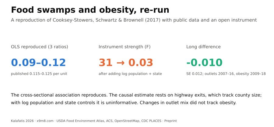
Cooksey-Stowers, Schwartz and Brownell (2017) reported that “food swamps”, counties with many fast-food outlets and convenience stores relative to grocery stores, predict adult obesity better than food deserts, and that an instrumental-variables (IV) estimate using highway exits was about 20 times the ordinary least squares (OLS) estimate. I reproduced the analysis from public data, replacing the commercial exit data with a count of OpenStreetMap motorway junctions. The published sample sizes, R² and control coefficients were reproduced closely once store counts were taken from 2007, not 2009 as the paper states. OLS coefficients were 0.086 to 0.120 percentage points of obesity per unit of the retail food environment index (published 0.115 to 0.125). IV estimates were positive (1.02 to 1.81; first-stage F 28 to 35). But motorway junctions correlate 0.90 with county population. With linear population or the count of people over 65 as controls, the instrument stayed strong (F 19 to 35) and estimates fell to 0.73 to 0.93; with log population and state fixed effects, the first-stage F fell to 0.03 and the Anderson–Rubin confidence set became unbounded. Within counties, changes in the index from 2007 to 2016 were not associated with changes in obesity from 2009 to 2018 (−0.010 per unit, SE 0.012), although noise and a change of obesity source may bias this toward zero. The cross-sectional association reproduces; the published IV estimate of 2.604 does not, and the causal estimate depends on how county size is controlled.
Keywords: food swamps; food deserts; retail food environment index; obesity; instrumental variables; weak instruments; reproducibility; OpenStreetMap
Social media summary: Food swamps and obesity, re-run: the link reproduces, but the causal estimate rests on highway exits that track county size.
1. Introduction
“Food swamp” describes a place where fast food and snack retail crowd out healthier options. Cooksey-Stowers, Schwartz and Brownell (2017) gave the idea its most cited quantitative test. Using county data for the United States, they related adult obesity to three versions of the retail food environment index (RFEI), the ratio of fast-food outlets and convenience stores to grocery stores, and to the share of residents with low income and low access to a supermarket, the usual food-desert measure. They found that “food swamps have a positive, statistically significant effect on adult obesity rates” even after controlling for food deserts, and that an IV estimate, with the number of highway exits in a county as the instrument, was much larger than the OLS estimate: 2.604 against 0.125 for the traditional RFEI. The discussion translated the IV coefficient into policy terms: zoning laws “could lower obesity rates by about three percent”. The publisher’s page showed 549 citations (the Google Scholar count) on 22 October 2026, and OpenAlex listed 642.
Three features of the paper make it worth re-running. First, the instrument came from a commercial street database (ESRI StreetMap North America) and no code was published; I found no published reproduction of the IV result. Second, highway exits are a familiar but contested instrument for food access. Dunn (2010) and Anderson and Matsa (2011) used interstate highways to shift restaurant supply, but the number of exits in a county also tracks its population, urbanisation and road network, all of which may affect obesity by other routes. The original’s limitations section acknowledged this: citing Dunn, it called highways “an imperfect instrument”, listed threats to the exclusion restriction and noted a “potentially weak instrument”. Third, the paper’s first-stage F statistics (7.87, 7.44 and 15.66) are in the range where conventional 2SLS t-tests are unreliable (Andrews et al., 2019; Lee et al., 2022), and no weak-instrument-robust intervals were reported.
The wider literature on local food environments and obesity is mixed. A systematic review found associations between food-outlet availability and obesity to be predominantly null, although indices combining several outlet types, like the RFEI, were the exposure most consistently associated with adult obesity (Cobb et al., 2015). Quasi-experimental studies have found effects of fast-food proximity in specific settings (Currie et al., 2010) and none in others (Anderson & Matsa, 2011). The food-swamp paper is widely cited and draws a direct policy conclusion for zoning, which makes it a useful target for a transparent reproduction.
This paper does four things. It reproduces the OLS and IV estimates from public data, documenting each choice and each point where the published description and the data disagree. It replaces the commercial exit counts with an open count of OpenStreetMap motorway junctions. It adds weak-instrument-robust inference, sensitivity checks on the ratio and the instrument, and a correct reading of the coefficient. And it updates the analysis with newer store counts and obesity estimates, including a county long difference that removes fixed differences between counties without needing an instrument. I did not contact the original authors.
2. Methods
2.1 Target estimates
The targets were read from the article’s HTML on mdpi.com and checked against its PDF; both carry the tables as text and give identical numbers. Table 6 of the original reports OLS coefficients of 0.120 (SE 0.0579), 0.115 (0.0499) and 0.125 (0.0443) for “Modified v1”, “Modified v2” and the traditional RFEI, with N = 3,069, 3,069 and 3,055 and R² of 0.559 to 0.560. Table 7 reports first-stage F statistics of 7.87, 7.44 and 15.66, and Table 8 IV coefficients of 1.510 (0.434), 1.277 (0.383) and 2.604 (1.076). Table 9 reports IV estimates for the traditional RFEI stratified by commuting mode and income inequality. Appendix Tables A4 and A5 add total food outlets as a control.
2.2 Data
Store and restaurant counts, recreation and fitness facilities, farmers’ markets, adult obesity, the food-desert measure, the Natural Amenities Index, the milk:soda price ratio and county demographics came from the USDA Economic Research Service Food Environment Atlas (U.S. Department of Agriculture, Economic Research Service [USDA ERS], 2025). Obesity is the age-adjusted percentage of adults aged 20 and over with BMI ≥ 30, as estimated by the CDC from the Behavioral Risk Factor Surveillance System for 2009. The paper states that it used “2009 data” and accessed the Atlas on 1 June 2015. The Atlas release current at that date (February 2014) carries store counts for 2007 and 2011, not 2009; 2009 counts appear in the November 2012 release, and the August 2015 release carries 2007 and 2012. I used the February 2014 release for 2007 counts (the November 2012 release carries slightly different 2007 counts, for example an SD of 228.48 rather than 228.58 for fast food) and the November 2012 release for 2009 counts, and ran the analysis with both (§3.1 explains why 2007 is the main specification).
The original merged demographic variables from the 2010 Census and the American Community Survey (ACS). I took % non-Hispanic Black, % Hispanic, the population aged 65 and over, median household income and the poverty rate from the Atlas, and the Gini index (table B19083), means of transport to work (B08301) and educational attainment (B15002) from the ACS 2006–2010 five-year estimates (U.S. Census Bureau, n.d.), retrieved from data.census.gov because the Census API now requires a key. The 2005–2009 ACS, which the original may have used, is not available through that service. Land area in square miles is the 2010 Census land area carried by the 2010 cartographic county boundary file, as redistributed in the plotly/datasets GitHub repository (Plotly, n.d.; commit 0c447c4).
2.3 Food-swamp measures
Following Table 1 of the original, with FFR the number of fast-food (limited-service) restaurants, CONVS convenience stores, GROC grocery stores and supermarkets, SUPERC supercenters and warehouse clubs, SPECS specialised food stores and FMRKT farmers’ markets:
- traditional RFEI = (FFR + CONVS) / GROC;
- expanded RFEI #1 = (FFR + CONVS + SUPERC) / (GROC + FMRKT + SPECS), supercenters counted as unhealthy;
- expanded RFEI #2 = (FFR + CONVS) / (GROC + FMRKT + SPECS + SUPERC), supercenters counted as healthy.
The RFEI has been used mainly at neighbourhood scale (Spence et al., 2009), and supercenters are hard to classify: Courtemanche and Carden (2011) estimated that Walmart Supercenters raise BMI and obesity, but supercenters also sell fresh food, and the original cited evidence in both directions. A ratio is undefined where its denominator is zero; in the main analysis those counties drop out, as they evidently did in the original. Sensitivity analyses kept them with an add-one ratio, (numerator + 1)/(denominator + 1), used its logarithm, dropped counties with denominators below 3, trimmed the top 1% of the ratio, and replaced the ratio with separate densities per 10,000 residents of unhealthy outlets (FFR + CONVS) and grocery stores (GROC); supercenters, specialised stores and farmers’ markets are left out of the densities.
2.4 Instrument
The original counted highway exits per county from ESRI StreetMap North America. As a public substitute I counted OpenStreetMap nodes tagged highway=motorway_junction, which mark numbered exits and interchanges on motorways, and assigned each to a county by point-in-polygon with the 2010 county boundaries (nodes within 2 km outside a generalised coastline were assigned to the nearest county). The nodes came from the QLever SPARQL engine (Bast & Buchhold, 2017) over the OpenStreetMap planet file of 21 September 2026 (OpenStreetMap contributors, 2026). For 16 states and the District of Columbia, which I had first downloaded from the Overpass API, the two sources agreed closely (22,986 against 23,073 nodes). A single interchange often has one node per carriageway, so I also counted distinct exit references per county. The substitute measures exits in 2026, not 2009; interchanges built since 2009 and changes in OpenStreetMap coverage add noise.
2.5 Models
The OLS model regresses county obesity on one RFEI and the controls. The 2SLS model instruments the RFEI with the exit count. The sample is the 3,108 counties of the contiguous United States, the coverage of the Natural Amenities Index, which matches the N = 3,108 of the original’s table titles. Following the text of the original, standard errors are clustered by state (49 clusters, including the District of Columbia), with the small-sample factor G/(G−1)·(N−1)/(N−K) used by Stata’s regress; Stata’s ivregress may differ slightly.
The notes to Tables 6–8 list the controls as the number of fitness centres, natural amenities, % Black, % Hispanic, the number of people over 65, the poverty rate and county size, alongside the food-desert measure and the milk:soda price ratio shown in the tables. That set reproduced the published R² poorly (§3.2). The covariates shown in the original’s Tables 9 and A4 (the same list with % bachelor’s degree in place of people over 65) reproduced it closely, and I used them as the main control set (food desert, recreation facilities, natural amenities, milk:soda price, % bachelor’s degree, % Black, % Hispanic, poverty rate, land area). Table 3 of the original reports a median of 12.2% for bachelor’s degree and 80.2% for driving to work, which are closer to the ACS shares with a bachelor’s degree only (11.7%) and driving alone (79.2%) than to bachelor’s or higher (16.9%) and any car travel (90.9%); I used those definitions.
2.6 Weak-instrument diagnostics and inference
For each 2SLS model I report the first-stage coefficient on the instrument and its Wald F statistic computed with the same clustered variance. With one instrument this equals the effective F of Montiel Olea and Pflueger (2013). Because 2SLS t-tests are unreliable when instruments are weak, and need a first-stage F of about 105 for a 5% t-test to have its nominal size (Lee et al., 2022), I also report Anderson–Rubin (AR) 95% confidence sets (Anderson & Rubin, 1949; Andrews et al., 2019), obtained by inverting the cluster-robust test of the instrument’s coefficient in a regression of obesity minus β times the RFEI on the instrument and controls. With one instrument the acceptance region solves a quadratic inequality, so the sets are exact; they can be bounded, the union of two rays, or the whole line. The instrument was varied (any exit, log of 1 + exits, exits per 1,000 square miles, distinct exit references), and controls for county size were added: the count of people over 65 named in the original’s table notes, population (linear), log population, log and linear population together, and state fixed effects. Cluster-robust inference follows Cameron and Miller (2015); conventional 2SLS inference is often unreliable in applied work with clustered or heteroskedastic errors (Young, 2022).
2.7 Update with newer data
The Food Environment Atlas released in July 2025 carries store counts for 2016 and 2020, but adult obesity only at state level for 2017 and 2022, and 2020 counts below three are coded −9999, so 2020 ratios cannot be formed for small counties. I used the 2016 counts (USDA ERS, 2025) and model-based, age-adjusted adult obesity prevalence for 2018 from CDC PLACES (2020 release; Centers for Disease Control and Prevention [CDC], n.d.; Greenlund et al., 2022), which applies multilevel regression and poststratification to BRFSS data (Zhang et al., 2014). The Atlas documentation defines −9999 as data “not available, not applicable, or suppressed”. The 2016 counts contain no zeros, so most −9999 codes are probably counties with no establishment of that type; treating them as zero is an assumption, and I checked the results in the 1,500 contiguous counties without any −9999-coded count. Controls were updated from the 2025 release or the ACS 2014–2018: food desert 2015, recreation facilities 2016, % Black, % Hispanic and people over 65 2020, poverty 2021, education 2014–2018; natural amenities, milk:soda price and land area were carried over. I ran the cross-section with OLS and 2SLS, then a long difference: the change in obesity between 2009 (Atlas) and 2018 (PLACES) regressed on the change in each RFEI between 2007 and 2016, with the 2010 controls and state fixed effects. The two obesity sources differ in method and age range (20+ against 18+), so state fixed effects absorb any state-level shift between them, and the long difference is read as a check on direction, not a precise estimate. Because the 2007 and 2016 indices are only moderately correlated (0.65 for the traditional RFEI), part of the measured change is noise, which would bias the long-difference slope toward zero.
2.8 Software, data and AI use
Analyses used Python 3.13 with pandas, NumPy, SciPy and GeoPandas; the regression and AR routines were written for this study and are in the package. Figures used matplotlib. The study was carried out with the assistance of Claude (Anthropic; model claude-opus-5-5) in October 2026, which retrieved data, wrote and ran the analysis code, read the original article, searched the literature and drafted the text under the author’s direction. Independent AI agents checked the numbers against the result files and the citations against their sources, and their corrections were applied. The author reviewed the work and takes full responsibility for it.
3. Results
3.1 Which data the original used
Table 3 of the original reports medians and standard deviations for the store counts. With the 2007 counts in the February 2014 release these match the published values to within 0.05: fast-food restaurants 15 (SD 228.58; published 228.60, and exactly 228.58 in Table 3’s separate row for the number of fast-food retailers), grocery stores 6 (76.81; 76.80), supercenters 0 (2.64; 2.64), convenience stores 16 (87.54; 87.50), specialised stores 1 (37.95; 37.95), and recreation facilities 2 (30.31; 30.31). The 2009 counts do not match (for example, fast food 14 with SD 230.52, and supercenters 1 with SD 3.36), and neither do the 2007 convenience-store counts in the August 2015 release (median 20, SD 255.72). The analytic sample sizes point the same way. In the contiguous United States, 53 counties had no grocery store in 2007 and 39 had no store of any kind in the expanded denominators, which leaves exactly 3,055 counties for the traditional RFEI and 3,069 for the expanded ones, the published Ns. With 2009 counts the Ns are 3,054, 3,064 and 3,065. Obesity (median 30.5, SD 4.16), the Natural Amenities Index, % Black, % Hispanic, median household income and the poverty rate also match the published descriptive statistics to the reported precision. Other variables are close but not identical: population (median 25,849 against 25,970), people over 65 (3,975 against 4,000), land area (604 against 624 square miles), bachelor’s degree (11.7% against 12.2%), driving alone (79.2% against 80.2%) and the Gini index (0.43 against 0.4), which fits the use of different Census or ACS vintages for these variables (results file reproduction.json). I therefore treat 2007 counts with 2009 obesity as the original’s data, and report 2009 counts as a variant.
3.2 OLS (Table 6)
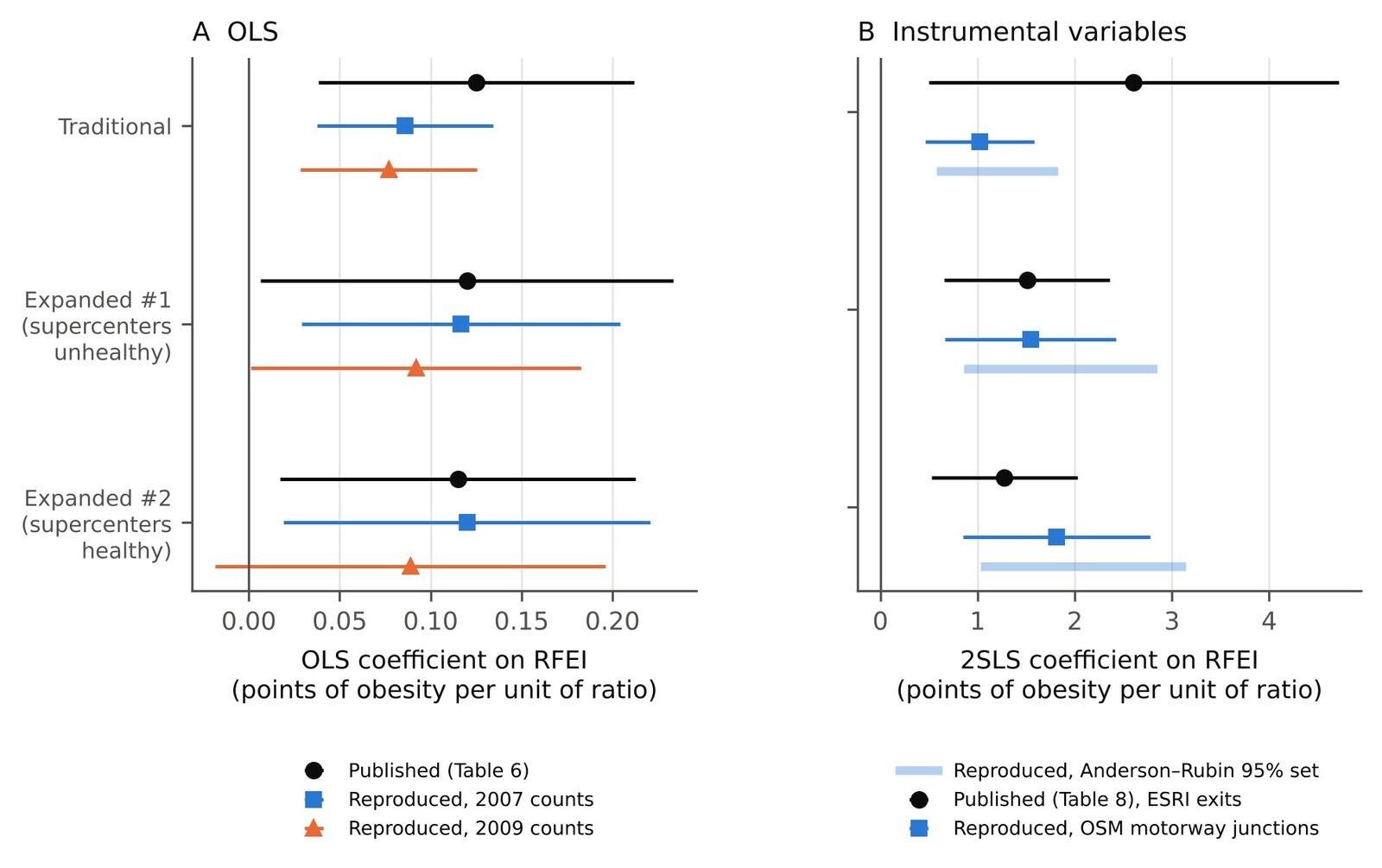
With 2007 counts and the main control set, the reproduction matched the published Table 6 closely (Table 1, Figure 1A). The R² was 0.560 for the traditional RFEI and 0.559 and 0.558 for the expanded ones (published 0.560, 0.559, 0.560). The control coefficients and their standard errors matched as well. For the traditional RFEI, natural amenities had a coefficient of −1.035 (state-clustered SE 0.198; published −1.039, SE 0.196), the milk:soda price ratio 1.560 (1.684; published 1.501, 1.670), the constant 34.06 (1.57; published 34.23, 1.573) and the food-desert measure 0.015 (0.015; published 0.0138, 0.0148). These SEs are clustered by state; heteroskedasticity-robust SEs are about three times smaller (0.059 for natural amenities). The original’s text describes “robust standard errors clustered by state”, and the reproduced SEs agree with that. The literal control list in the table notes, with people over 65 in place of % bachelor’s degree, gave an R² of 0.474.
The expanded RFEI coefficients were 0.117 (SE 0.045) for #1 and 0.120 (0.051) for #2. The published values were 0.120 (0.0579) for “Modified v1” and 0.115 (0.0499) for “Modified v2”. The labels are ambiguous in the original: Table 1, §2.2.2 and Table 4 put supercenters in the numerator of #1 and the denominator of #2, while the note to Table 3 and the list in §2.4.1 say the reverse, and §3.3 describes “expanded RFEI 1 with supercenters categorized as healthy”. The reproduced #2 is closest to the published v1, and the reproduced #1 to v2, which fits the Table 3 note; the published SDs (2.14 and 2.38 against 2.17 and 2.41 reproduced) point the same way. Either way the expanded coefficients reproduce to within 0.01, but the published expanded-index medians and Table 4 counts are not reproduced exactly by either definition (for example, a median of 3.4 against 3.76 for #1).
The traditional RFEI did not reproduce as well: 0.086 (SE 0.025) against 0.125 (0.0443). The published descriptive statistics suggest why. Table 3 of the original gives the traditional RFEI a median of 3.5 and SD of 1.86, and Table 4 a mean of 3.89. With the same data (all counties), the Table 1 formula gives a median of 5.33, SD of 3.54 and mean of 5.84. I searched 1,372 constructions, every sum of one to four outlet types over every sum of one to three healthy outlet types (script 07_construction_search.py). One construction matches all three published values: (CONVS + GROC)/GROC, with median 3.50 and SD 1.86 across all counties and mean 3.92 in the 3,108 contiguous counties; the next closest has an SD of 1.77. It does not reproduce the Table 4 count of counties above 3.89 (1,244 against 1,419), and neither does any other construction. Its OLS coefficient is 0.132 (SE 0.045), close to the published 0.125 (0.0443), with R² 0.558. This is consistent with grocery stores having entered the numerator in place of fast-food outlets, which would make the published “traditional RFEI” equivalent in regression to convenience stores per grocery store, plus one. I cannot confirm this without the original code or data, and I report both constructions.
Table 1. Published and reproduced estimates of the food-swamp coefficient (percentage points of adult obesity per one-unit change in the RFEI ratio). Reproduction: 2007 store counts, 2009 obesity, contiguous US counties, controls for % low income and low access, recreation and fitness facilities, natural amenities, milk:soda price ratio, % bachelor’s degree, % Black, % Hispanic, poverty rate and land area; standard errors clustered by state. Instrument: published, ESRI StreetMap highway exits; reproduced, OpenStreetMap motorway junctions (2026). Published labels “Modified v1/v2” are placed against the Table 1 definitions; see §3.2 for the label ambiguity.
| RFEI | Published OLS (SE) | Reproduced OLS (SE) | N pub. / rep. | R² pub. / rep. | Published IV (SE) | Reproduced IV (SE) | First-stage F pub. / rep. | Reproduced AR 95% set |
|---|---|---|---|---|---|---|---|---|
| Traditional | 0.125 (0.0443) | 0.086 (0.0247) | 3,055 / 3,055 | 0.560 / 0.560 | 2.604 (1.076) | 1.023 (0.285) | 15.66 / 30.7 | [0.58, 1.82] |
| Expanded #1 (supercenters unhealthy) | 0.120 (0.0579) | 0.117 (0.0447) | 3,069 / 3,069 | 0.559 / 0.559 | 1.510 (0.434) | 1.544 (0.449) | 7.87 / 27.5 | [0.86, 2.85] |
| Expanded #2 (supercenters healthy) | 0.115 (0.0499) | 0.120 (0.0515) | 3,069 / 3,069 | 0.560 / 0.558 | 1.277 (0.383) | 1.811 (0.491) | 7.44 / 35.0 | [1.03, 3.14] |
| (CONVS + GROC)/GROC, see §3.2 | — | 0.132 (0.0454) | — / 3,055 | — / 0.558 | — | 3.257 (1.539) | — / 6.9 | [1.45, 14.66] |
3.3 The open instrument
OpenStreetMap had 77,175 motorway-junction nodes in the contiguous counties; 1,142 of the 3,108 counties had none, against 1,672 with no exit in the original. The open count resembles the original instrument in how it relates to other county characteristics. Its correlation with obesity was −0.21 (published −0.20), with fast-food restaurants 0.90 (0.86), with recreation facilities 0.87 (0.84), with population 0.90 (0.86) and with land area 0.12 (0.14). The original reports a negative correlation with the traditional RFEI (−0.07); the open count’s correlation was 0.07 with the Table 1 construction.
3.4 IV (Tables 7 and 8)
With the open instrument and the main controls, all three 2SLS estimates were positive and well above OLS (Table 1, Figure 1B): 1.02 (SE 0.29) for the traditional RFEI, 1.54 (0.45) for expanded #1 and 1.81 (0.49) for expanded #2. The first-stage F statistics were 30.7, 27.5 and 35.0, stronger than the published 15.66, 7.87 and 7.44, and the AR 95% sets were bounded: [0.58, 1.82], [0.86, 2.85] and [1.03, 3.14]. The expanded estimates are close to or somewhat above the published 1.510 and 1.277. The traditional estimate is less than half the published 2.604. For the (CONVS + GROC)/GROC construction, the 2SLS estimate was 3.26 (SE 1.54), with a first-stage F of 6.9 and an AR set of [1.45, 14.66], which is closer to the published value and, like it, rests on a weak first stage.
3.5 What the instrument identifies
The open count of motorway junctions tracks county size: its correlation with 2010 population is 0.90 (Figure 2A), and each junction is associated with 0.36 more recreation facilities (SE 0.04) after the other controls. The published control lists do not include population; the original’s controls are shares, a count of fitness centres and, in the table notes, the count of people over 65, which correlates 0.98 with population. How much of the instrument survives depends on how size is controlled (Table 2, Figure 2B). With the count of people over 65 the first stage stayed strong (F 35.4; 2SLS 0.93, SE 0.23), and so it did with population entered linearly (F 19.3; 2SLS 0.73, SE 0.25; AR set [0.33, 1.46]) or linearly with state fixed effects (F 33.6; 0.53, SE 0.17). With log population the first-stage F fell to 4.8 and the AR set widened to [0.79, 16.47]; with log and linear population together, to 4.0; and with log population and state fixed effects, to 0.03, with an unbounded AR set. The expanded indices behaved the same way (F 0.41 and 0.48 with log population and state fixed effects). State fixed effects alone did not weaken the instrument (F 41.9; 2SLS 0.77, SE 0.18).
I take log population as the more appropriate size control, because exits and population are related on the log scale (Figure 2A) and a linear term is dominated by a few very large counties; with log population included, adding the linear term does not restore the first stage. On that reading, the instrument’s strength comes from differences in county size within states. Larger, more urban counties have more exits, more fast-food outlets per grocery store and, conditional on the other controls, different obesity rates for many reasons, so the exclusion restriction is hard to defend. A reader who prefers a linear size control would conclude that the instrument is strong and the effect positive but smaller (0.53 to 0.93), still well below the published 2.604. Either way, the original’s own over-65 control would not have removed the first stage in this reproduction.
How the exits enter the first stage also mattered (Table 2, Figure 3). With a binary indicator for any exit the 2SLS estimate for the traditional RFEI was 0.28 (SE 0.14); with log(1 + exits), 0.34 (0.14); with distinct exit references, 1.07 (0.43; F 6.9); and with exits per 1,000 square miles, a density that does not scale with population, the first stage was weak (F 1.8) and the AR set unbounded. Restricting to the 1,954 counties with at least one exit gave 1.28 (0.40). Across specifications in which the instrument was strong (F above 10), leaving aside the log-ratio specification, which is in different units, the 2SLS estimates ranged from 0.28 to 1.34 per unit of the traditional RFEI, all below the published 2.604.
Table 2. Sensitivity of the traditional-RFEI estimates. OLS and 2SLS coefficients (state-clustered SE), first-stage F on the excluded instrument (state-clustered; with one instrument this equals the Montiel Olea–Pflueger effective F) and Anderson–Rubin 95% confidence sets. The log specification is in log units and not comparable in size with the others.
| Specification | N | OLS (SE) | 2SLS (SE) | First-stage F | AR 95% set |
|---|---|---|---|---|---|
| Baseline (2007 counts, matched controls, clustered SE) | 3,055 | 0.086 (0.025) | 1.02 (0.29) | 30.71 | [0.58, 1.82] |
| 2009 store counts | 3,054 | 0.077 (0.025) | 1.01 (0.31) | 21.14 | [0.55, 1.99] |
| State fixed effects | 3,055 | 0.063 (0.017) | 0.77 (0.18) | 41.91 | [0.46, 1.21] |
| Add people over 65 (count, as in the table notes) | 3,054 | 0.085 (0.025) | 0.93 (0.23) | 35.44 | [0.56, 1.54] |
| Add population (linear) | 3,055 | 0.083 (0.025) | 0.73 (0.25) | 19.30 | [0.33, 1.46] |
| Add population (linear) + state fixed effects | 3,055 | 0.062 (0.017) | 0.53 (0.17) | 33.62 | [0.21, 0.92] |
| Add log population | 3,055 | 0.066 (0.024) | 1.76 (0.87) | 4.83 | [0.79, 16.47] |
| Add log and linear population | 3,055 | 0.065 (0.025) | 1.17 (0.61) | 3.98 | [0.43, 57.10] |
| Add log population + state fixed effects | 3,055 | 0.043 (0.018) | 15.58 (92.13) | 0.03 | unbounded (two rays) |
| Population-weighted | 3,054 | 0.228 (0.049) | 1.34 (0.28) | 105.93 | [0.83, 1.95] |
| Zero denominators kept: (num+1)/(den+1) | 3,108 | 0.130 (0.039) | 0.97 (0.26) | 35.18 | [0.55, 1.69] |
| Drop counties with denominator < 3 | 2,492 | 0.137 (0.030) | 1.00 (0.28) | 32.63 | [0.57, 1.77] |
| Drop top 1% of RFEI | 3,024 | 0.104 (0.028) | 1.10 (0.34) | 25.33 | [0.60, 2.11] |
| Log of (num+1)/(den+1) | 3,108 | 0.527 (0.186) | 5.02 (1.17) | 49.08 | [3.03, 7.92] |
| Instrument: any exit (0/1) | 3,055 | 0.086 (0.025) | 0.28 (0.14) | 67.07 | [0.04, 0.60] |
| Instrument: log(1 + exits) | 3,055 | 0.086 (0.025) | 0.34 (0.14) | 44.16 | [0.09, 0.68] |
| Instrument: exits per 1,000 sq mi | 3,055 | 0.086 (0.025) | 1.80 (1.01) | 1.82 | unbounded (two rays) |
| Instrument: distinct exit refs | 3,055 | 0.086 (0.025) | 1.07 (0.43) | 6.87 | [0.51, 4.00] |
| Counties with at least one exit | 1,954 | 0.108 (0.026) | 1.28 (0.40) | 15.15 | [0.72, 2.74] |

3.6 Zero denominators and the shape of the ratio
Ratios with small denominators are unstable. Keeping the 53 counties without a grocery store by adding one to numerator and denominator raised the OLS coefficient to 0.130 (SE 0.039; N = 3,108); dropping counties with fewer than three grocery stores raised it to 0.137 (0.030; N = 2,492); weighting by population raised it to 0.228 (0.049). The 2SLS estimates moved less, between 0.97 and 1.34. When the ratio was split into unhealthy-outlet and grocery-store densities, the sign of the unhealthy component changed: in the same OLS model, each additional fast-food outlet or convenience store per 10,000 residents was associated with 0.025 fewer percentage points of obesity (SE 0.014), and each additional grocery store per 10,000 with 0.124 fewer (0.042). The positive RFEI coefficient appears to be driven mainly by the grocery-store denominator rather than by more fast food per person, although the unhealthy-density coefficient is imprecise (p ≈ 0.08) and this decomposition is descriptive.
3.7 Stratified IV (Table 9)
Table 9 of the original splits counties at 80% driving or taking public transport to work and at a Gini index of 0.41. With the ACS 2006–2010 data, 1,510 counties fell below 80% on driving alone plus public transport (published 1,230), and 847 fell below a Gini of 0.41 (published 2,442); a split leaving 2,442 counties below would need a cut-off near 0.46. In the low-commuting group the 2SLS estimate was 1.43 (SE 0.67), but the first-stage F was 3.8 and the AR set unbounded, the union of two rays (−∞, −621.8] ∪ [0.75, ∞). In the high-commuting group it was 0.98 (0.31; F 10.9). For Gini below 0.41 the first stage was very weak (F 1.8, AR set the union of two rays); above 0.41, 0.98 (0.28; F 31.3). The original’s abstract and Table 9 disagree on direction: the abstract says the effect was “stronger in counties with greater income inequality (p < 0.05)”, while Table 9 reports 2.737 for Gini below 0.41 and 1.564 above, and the original’s results text agrees with Table 9 (“remained statistically significant in areas with lower income inequality”). The abstract also gives p < 0.01 for less mobile counties, where Table 9 marks the estimate p < 0.05. No stratified estimate here had a strong first stage in both halves.
3.8 Newer data
With 2016 store counts and PLACES obesity for 2018, the cross-sectional pattern repeated (Table 3). For the traditional RFEI, OLS gave 0.056 (SE 0.030) and 2SLS 0.87 (0.26) with a first-stage F of 21.4, or 0.46 (0.20; F 15.3) with state fixed effects. Adding log population with state fixed effects again removed the instrument’s strength (F 0.63, AR set unbounded). Excluding counties with any −9999-coded count left 1,500 counties. There the traditional RFEI gave 2SLS 2.27 (SE 1.12) on a weak first stage (F 4.1), but the expanded indices gave 2.11 (0.71; F 11.7) and 2.24 (0.68; F 17.0) on strong ones, close to the published IV estimates. Those counties are larger (all their outlet types are present), and these estimates were not checked against size controls.
The long difference points the other way. Mean county obesity rose by 4.9 points between 2009 and 2018 (SD 3.1). Conditional on state fixed effects and 2010 controls, the change in the traditional RFEI between 2007 and 2016 had a coefficient of −0.010 (SE 0.012; N = 3,011). For the expanded indices the coefficients were −0.012 (0.015) and 0.002 (0.020). These estimates exclude the cross-sectional OLS coefficient of 0.086 and the open-instrument 2SLS coefficient of 1.02. Adding changes in poverty and education did not alter them, and restricting to counties without −9999-coded counts gave −0.027 (0.021) for the traditional RFEI and −0.082 (0.047) and −0.062 (0.052) for the expanded ones. Counties whose outlet mix shifted towards fast food and convenience stores did not see faster growth in obesity. Two caveats limit this. The 2007 and 2016 indices correlate only 0.65 (0.63 and 0.62 for the expanded ones), so the change is measured with noise that biases the slope toward zero; and the outcome change mixes two estimation methods, which state fixed effects absorb only at state level. An effect could also take longer than a decade to appear.
Table 3. Update with newer data. Cross-section: 2016 store counts (Food Environment Atlas, July 2025 release; −9999 codes treated as zero) and model-based adult obesity for 2018 (CDC PLACES, 2020 release), contiguous US counties, controls updated where available (food desert 2015, recreation facilities 2016, % Black, % Hispanic and people over 65 2020, poverty 2021, education ACS 2014–2018), OSM instrument. “No −9999” restricts to the 1,500 counties without any −9999-coded count. Long difference: change in obesity 2009→2018 regressed on change in the RFEI 2007→2016, with 2010 baseline controls and state fixed effects. State-clustered SE.
| RFEI | Cross-section OLS (SE) | Cross-section 2SLS (SE) | First-stage F | 2SLS + state FE (SE) | First-stage F, FE | 2SLS, no −9999 (SE) | First-stage F, no −9999 | Long difference (SE) | N (long difference) |
|---|---|---|---|---|---|---|---|---|---|
| Traditional | 0.056 (0.030) | 0.87 (0.26) | 21.4 | 0.46 (0.20) | 15.3 | 2.27 (1.12) | 4.1 | -0.010 (0.012) | 3,011 |
| Expanded #1 (supercenters unhealthy) | 0.096 (0.059) | 1.37 (0.43) | 24.8 | 0.76 (0.35) | 11.9 | 2.11 (0.71) | 11.7 | -0.012 (0.015) | 3,034 |
| Expanded #2 (supercenters healthy) | 0.105 (0.075) | 1.70 (0.55) | 27.8 | 0.95 (0.46) | 9.7 | 2.24 (0.68) | 17.0 | 0.002 (0.020) | 3,035 |

3.9 Reading the coefficient
The RFEI coefficient is the change in obesity, in percentage points, per one-unit change in a ratio of outlet counts. It is not an elasticity. The original reads the OLS coefficient as meaning that “a 1 percent increase in fast food restaurants increases obesity by approximately 0.125 percent”. Under the Table 1 construction, a 1% increase in fast-food outlets raises the traditional RFEI by 1% of FFR/GROC, which is 0.027 units in the median county. At the published coefficient of 0.125, that is 0.0033 percentage points of obesity, an elasticity at the means of about 0.012. The original’s own discussion gives a similar lower figure, saying the OLS estimates imply that mitigating food swamps would lower obesity “by about 0.003 to 0.12 percent”. (Under the (CONVS + GROC)/GROC construction, fast food would not enter the index at all.) For the IV coefficient, the size of one standard deviation depends on the construction. With the published SD of 1.86, which §3.2 argues belongs to the index actually used, 2.604 per unit implies 4.8 points per SD, about 1.2 SD of county obesity (4.16); with the Table 1 construction (SD 3.53 in the regression sample), 9.2 points. The original says zoning “could lower obesity rates by about three percent”. If that is read as three percentage points, which is my interpretation, it requires lowering the RFEI by 1.15 units at 2.604 per unit: in the median county, removing about 7 fast-food outlets or convenience stores, 21% of them, or adding the equivalent grocery stores. Read as 3% of the mean obesity rate (30.3%), it is about 0.9 points.
4. Discussion
4.1 What reproduces and what does not
The descriptive and OLS parts of Cooksey-Stowers et al. (2017) reproduce from public data once the store counts are taken from 2007. Sample sizes, R² and the control coefficients match closely, and the expanded-RFEI coefficients agree to within 0.01. There is a robust, modest, positive cross-sectional association between the ratio of fast-food and convenience outlets to grocery stores and county adult obesity. That is a fair reading of the original’s OLS tables.
The causal claim is harder to sustain. An open substitute for the highway-exit instrument behaved much like the original in its correlations with county characteristics and produced positive IV estimates, with bounded AR sets. But its strength is tied to county size. Once log population and state are held fixed, it has no predictive power for the food environment and the data are consistent with any effect size. With a linear size control it stays strong, and the estimates fall to roughly 20–36% of the published 2.604. The size of the IV estimate also depended on how exits were coded, by a factor of about four. The long difference, which needs no instrument, found no association between changes in the outlet mix and changes in obesity over roughly a decade, though it is attenuated by noise and mixes obesity sources. Taken together, these results suggest that much of the gap between OLS and IV in the original reflects what highway exits measure, not only the correction of a downward bias from residential sorting.
These conclusions are mine and are conditional on the substitute instrument and on the choice of size control. The original’s ESRI exit counts may differ from OpenStreetMap junctions in ways that matter, though the similar correlations with population, fast food, recreation facilities and obesity suggest that they measure much the same thing. The original’s own first-stage F statistics (7.44 to 15.66) were lower than the ones here and below the thresholds now recommended for 2SLS t-tests (Lee et al., 2022), so the published IV confidence intervals were probably too narrow even on their own terms.
4.2 Documentation
Several discrepancies are listed in Table 4: the year of the store counts, the construction of the traditional RFEI, the placement of supercenters, the control set named in the table notes, the food-desert spread and the milk:soda price ratio in Table 3, and the abstract’s statements on inequality and mobility, which differ from Table 9 and the original’s own results text. Table 4 also records one clarification: the table notes’ “robust standard errors” are the state-clustered errors described in the text. None of these is unusual in observational research, and some may be typographical. The second matters most. If the published traditional RFEI was (CONVS + GROC)/GROC, the headline coefficients for the traditional index describe convenience stores relative to grocery stores, not fast food. The expanded indices, which do contain fast food, gave similar OLS coefficients, so the qualitative OLS finding does not depend on it. Sharing code and the merged data file would have resolved these points quickly, which is the case for open materials rather than a criticism of these authors in particular.
Table 4. Points where the published description and the public data diverge, with the evidence from this reproduction.
| Item | Published | What the data show |
|---|---|---|
| Year of store counts | “2009 data” (§2.1) | Table 3 medians (SD) match the 2007 counts in the February 2014 release to within 0.05: fast food 15 (228.58; Table 3’s row “Number of fast food retailers” gives 228.58 exactly), grocery 6 (76.81), specialised 1 (37.95), recreation 2 (30.31); the analytic Ns 3,055 and 3,069 arise with 2007 counts (3,055, 3,069) but not 2009 counts (3,054, 3,064); the August 2015 release’s 2007 convenience-store counts differ (median 20, SD 255.72) |
| Traditional RFEI | (FFR + CONVS)/GROC (Table 1) | That ratio has median 5.33, SD 3.54; the published 3.5 (1.86) and Table 4 mean 3.89 are matched by (CONVS + GROC)/GROC, the closest of 1,372 constructions searched: median 3.50, SD 1.86, mean 3.92 (contiguous counties). The Table 4 count above 3.89 (1,419) is not reproduced (1,244) |
| Supercenter placement | Table 1, §2.2.2 and Table 4: #1 numerator, #2 denominator; Table 3 note and §2.4.1: the reverse; §3.3 calls #1 “supercenters categorized as healthy” | Reproduced OLS for the Table 1 #2 definition is closest to the published v1 coefficient, and vice versa; the published expanded-index medians, SDs and Table 4 counts are not reproduced exactly by either definition |
| Control set, Tables 6–8 | Notes list % Black, % Hispanic, people over 65, poverty, county size | The note set gives R² 0.474; replacing people over 65 with % bachelor’s (as in Tables 9 and A4) gives R² 0.560 (published 0.560) and matches the published control coefficients |
| Standard errors (clarification, not a discrepancy) | Table notes: “robust”; §3.3: “robust standard errors clustered by state” | Consistent: published SEs for the controls match state-clustered SEs (e.g. natural amenities 0.196 vs 0.198 reproduced) |
| Food-desert spread | Table 3: 6.2 (8.37) | 8.37 is the mean (8.37); the SD is 8.21 |
| Milk:soda price ratio | Table 3: 30.2 (62.10) | The Atlas ratio has median 0.845 and SD 0.126 |
| Abstract vs Table 9 | Abstract: effect “stronger in counties with greater income inequality (p < 0.05)” and where residents are less mobile “(p < 0.01)” | Table 9 gives 2.737 for Gini < 0.41 and 1.564 for Gini > 0.41 (larger where inequality is lower), and the original’s §3.4 text agrees with Table 9; the low-mobility estimate is marked p < 0.05. With the ACS 2006–2010 Gini, 847 of 3,055 counties are below 0.41; a split with 2,442 below would need a cut-off near 0.46 |
4.3 Interpretation and policy
The original’s sentence reading the coefficient as an elasticity misstates its units and size: a level-on-ratio coefficient of 0.125 corresponds to a few thousandths of a percentage point per 1% change in fast-food outlets, a figure the original’s discussion also gives as its lower bound. The IV coefficient, read per standard deviation, implies effects of 1.2 to 2.2 standard deviations of county obesity, which is large for a single feature of the retail environment and consistent with 2SLS amplifying something other than the food environment. Neither result is evidence against food-environment policy as such. Zoning, healthy-retail incentives and outlet restrictions may still be worth trying, but evaluations should rest on designs that use changes over time or policy variation, not on the county cross-section with highway exits.
The density results add a further caution. Measured per resident, fast-food and convenience outlets were not positively associated with obesity, while grocery stores per resident were negatively associated (supercenters, specialised stores and farmers’ markets were left out of these densities). A ratio of counts mixes these, and it is driven by the number of grocery stores in small counties. Ratios with small denominators can produce associations that reflect the denominator more than the numerator, which argues for reporting the components alongside any index.
4.4 Limitations
The substitute instrument measures 2026 exits, and OpenStreetMap coverage is uneven, so it cannot reproduce the original’s IV estimates exactly; the conclusions about the IV rest on how the open instrument behaves, and on the published first-stage statistics. The ACS 2006–2010 estimates differ slightly from the 2005–2009 estimates the original may have used, which affects the Gini and commuting splits in Table 9. The obesity data are model-based county estimates from self-reported height and weight, and PLACES estimates use county demographic composition in their models (Zhang et al., 2014), which can induce associations with demographic covariates. The long difference compares two obesity sources with different methods and age ranges; state fixed effects remove state-level shifts between them but not county-specific ones, the change in the index is measured with noise (2007–2016 correlation 0.65), and both bias the slope toward zero. The 2016 counts treat codes of −9999 as zeros, an assumption. The update uses counts from 2016, because 2020 counts below three are coded −9999. The choice between log and linear population as the size control decides whether the open instrument is informative, and the data alone do not settle it. All analyses are ecological: county associations do not show what happens to individuals. The control set was chosen to match the published estimates, and I did not try every alternative.
5. Conclusion
The cross-sectional association between food swamps and county obesity reported by Cooksey-Stowers, Schwartz and Brownell (2017) reproduces from public data, with the store counts taken from 2007. The instrumental-variables estimate of 2.604 was not reproduced: with an open substitute for the highway-exit instrument the estimates were smaller, and they depended on how county size was controlled, from about 0.5 to 0.9 with linear size controls to uninformative with log population and state fixed effects. The original’s zoning figure of “about three percent”, which rests on the IV estimate, inherits that uncertainty. Highway exits track how big a county is, and a long difference with newer data, though attenuated, found no association between changes in the outlet mix and changes in obesity. Food-environment policy may still be worth pursuing, but the evidence for it needs designs that follow places over time.
Related on x9m8
- Drive-thru dose–response: GLP-1 uptake and US restaurant employment, paper 11
- Eating less, eating differently: the cost of an adequate diet on GLP-1 drugs, paper 10
- Validated, Not Confirmed: The Track Record of Statistically Validated Exoplanets, another reproducibility paper
Acknowledgements
The author thanks the USDA Economic Research Service, the US Census Bureau, the CDC PLACES team, the OpenStreetMap contributors and the QLever team for public data and services, and Cooksey-Stowers, Schwartz and Brownell for a paper detailed enough to reproduce. Claude (Anthropic; model claude-opus-5-5) assisted with data retrieval, analysis code, literature search and drafting in October 2026, as described in §2.8. The author reviewed all outputs and is responsible for the content.
Author contributions
P.K. conceived the study, directed the analysis, and reviewed and approved the manuscript.
Financial support
This research received no specific grant from any funding agency, commercial or not-for-profit sector.
Conflicts of interest
The author operates a restaurant, The Heritage Diner, in Mount Sinai, New York. Restaurants are part of the food environment studied here, and the findings concern fast-food outlets among others. The author declares no other financial interest in the food, restaurant or retail industries.
Research transparency and reproducibility
All data are public: USDA ERS Food Environment Atlas releases of November 2012, February 2014 and July 2025; ACS five-year tables from data.census.gov; CDC PLACES county data (2020 release); OpenStreetMap data via QLever; and 2010 county boundaries from plotly/datasets. Code, derived result files and the list of source URLs are in the reproducibility package linked from the article page. Raw third-party files are not redistributed. The analysis was not preregistered.
References
Anderson, M. L., & Matsa, D. A. (2011). Are restaurants really supersizing America? American Economic Journal: Applied Economics, 3(1), 152–188. https://doi.org/10.1257/app.3.1.152
Anderson, T. W., & Rubin, H. (1949). Estimation of the parameters of a single equation in a complete system of stochastic equations. The Annals of Mathematical Statistics, 20(1), 46–63. https://doi.org/10.1214/aoms/1177730090
Andrews, I., Stock, J. H., & Sun, L. (2019). Weak instruments in instrumental variables regression: Theory and practice. Annual Review of Economics, 11(1), 727–753. https://doi.org/10.1146/annurev-economics-080218-025643
Bast, H., & Buchhold, B. (2017). QLever: A query engine for efficient SPARQL+Text search. In Proceedings of the 2017 ACM on Conference on Information and Knowledge Management (pp. 647–656). Association for Computing Machinery. https://doi.org/10.1145/3132847.3132921
Cameron, A. C., & Miller, D. L. (2015). A practitioner’s guide to cluster-robust inference. Journal of Human Resources, 50(2), 317–372. https://doi.org/10.3368/jhr.50.2.317
Centers for Disease Control and Prevention. (n.d.). PLACES: County data (GIS friendly format), 2020 release [Data set]. Retrieved October 22, 2026, from https://data.cdc.gov/resource/mssc-ksj7.csv
Cobb, L. K., Appel, L. J., Franco, M., Jones-Smith, J. C., Nur, A., & Anderson, C. A. M. (2015). The relationship of the local food environment with obesity: A systematic review of methods, study quality, and results. Obesity, 23(7), 1331–1344. https://doi.org/10.1002/oby.21118 (Erratum published 2015, Obesity, 23(12), 2517–2519, https://doi.org/10.1002/oby.21363)
Cooksey-Stowers, K., Schwartz, M. B., & Brownell, K. D. (2017). Food swamps predict obesity rates better than food deserts in the United States. International Journal of Environmental Research and Public Health, 14(11), Article 1366. https://doi.org/10.3390/ijerph14111366
Courtemanche, C., & Carden, A. (2011). Supersizing supercenters? The impact of Walmart Supercenters on body mass index and obesity. Journal of Urban Economics, 69(2), 165–181. https://doi.org/10.1016/j.jue.2010.09.005
Currie, J., DellaVigna, S., Moretti, E., & Pathania, V. (2010). The effect of fast food restaurants on obesity and weight gain. American Economic Journal: Economic Policy, 2(3), 32–63. https://doi.org/10.1257/pol.2.3.32
Dunn, R. A. (2010). The effect of fast-food availability on obesity: An analysis by gender, race, and residential location. American Journal of Agricultural Economics, 92(4), 1149–1164. https://doi.org/10.1093/ajae/aaq041
Greenlund, K. J., Lu, H., Wang, Y., Matthews, K. A., LeClercq, J. M., Lee, B., & Carlson, S. A. (2022). PLACES: Local data for better health. Preventing Chronic Disease, 19, Article 210459. https://doi.org/10.5888/pcd19.210459
Lee, D. S., McCrary, J., Moreira, M. J., & Porter, J. (2022). Valid t-ratio inference for IV. American Economic Review, 112(10), 3260–3290. https://doi.org/10.1257/aer.20211063
Montiel Olea, J. L., & Pflueger, C. (2013). A robust test for weak instruments. Journal of Business & Economic Statistics, 31(3), 358–369. https://doi.org/10.1080/00401706.2013.806694
OpenStreetMap contributors. (2026). OpenStreetMap planet file, 21 September 2026 [Data set; Open Database License 1.0]. Queried via QLever, https://qlever.dev/api/osm-planet
Plotly. (n.d.). geojson-counties-fips.json [Data set; 2010 Census cartographic county boundaries]. plotly/datasets, commit 0c447c47b757ad74edecab31f0d72f849d2e67c2. GitHub. https://github.com/plotly/datasets
Spence, J. C., Cutumisu, N., Edwards, J., Raine, K. D., & Smoyer-Tomic, K. (2009). Relation between local food environments and obesity among adults. BMC Public Health, 9, Article 192. https://doi.org/10.1186/1471-2458-9-192
U.S. Census Bureau. (n.d.). American Community Survey 5-year estimates, 2006–2010 and 2014–2018, Tables B01003, B08301, B15002 and B19083 [Data set]. Retrieved October 22, 2026, from https://data.census.gov/
U.S. Department of Agriculture, Economic Research Service. (2025). Food Environment Atlas [Data set; current release of July 2025 and archived releases of November 2012 and February 2014]. https://www.ers.usda.gov/data-products/food-environment-atlas/data-access-and-documentation-downloads
Young, A. (2022). Consistency without inference: Instrumental variables in practical application. European Economic Review, 147, Article 104112. https://doi.org/10.1016/j.euroecorev.2022.104112
Zhang, X., Holt, J. B., Lu, H., Wheaton, A. G., Ford, E. S., Greenlund, K. J., & Croft, J. B. (2014). Multilevel regression and poststratification for small-area estimation of population health outcomes: A case study of chronic obstructive pulmonary disease prevalence using the Behavioral Risk Factor Surveillance System. American Journal of Epidemiology, 179(8), 1025–1033. https://doi.org/10.1093/aje/kwu018




[…] Automata Explained: Game of Life, Rule 30 and Rule 110, With a Simulator You Can Run • Food swamps and obesity revisited: a reproduction with public data […]
[…] Food swamps and obesity revisited: a reproduction with public data, the series’ first reproduction […]
[…] Food swamps and obesity revisited: a reproduction with public data […]
[…] Food swamps and obesity revisited: a reproduction with public data […]