Fluid Simulator: Stir the Navier–Stokes Equations in a Browser Tab

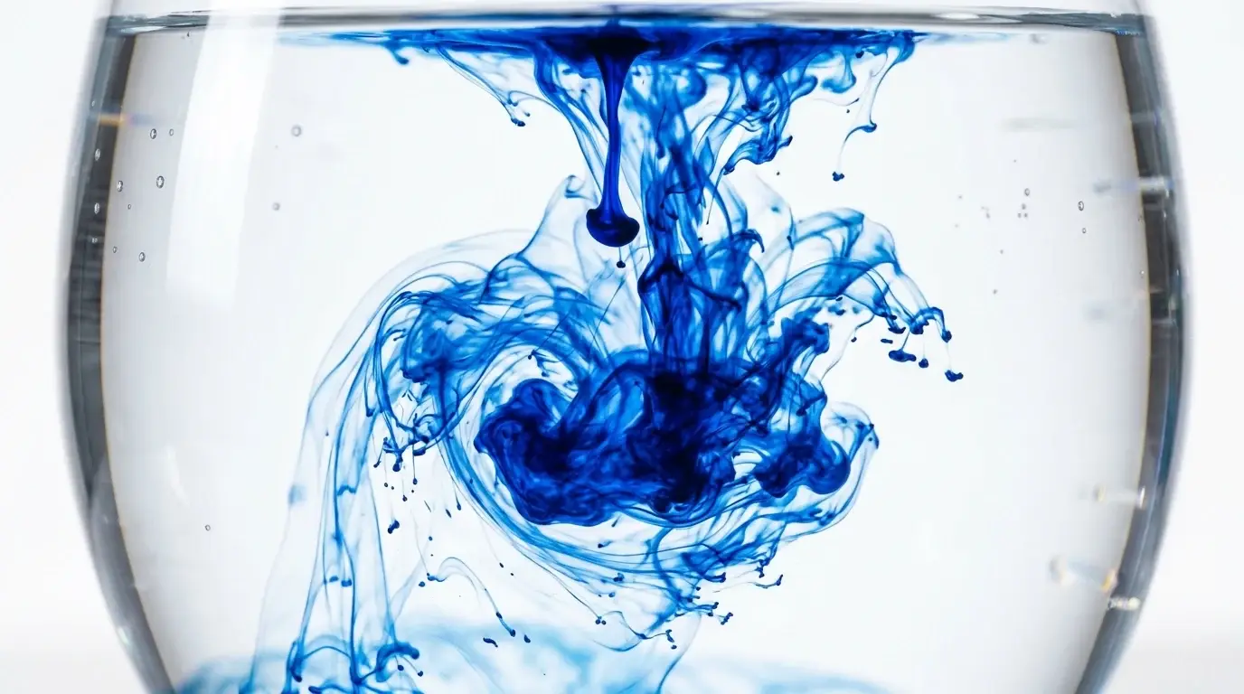
Drag the mouse across the canvas and a streak of dye curls into a vortex, sheds a second one, and keeps swirling after the mouse has stopped. The simulation behind it solves the same equations that govern smoke, weather and blood flow, on a grid, sixty times a second, on whatever graphics chip is in the machine reading this. The method is Jos Stam’s Stable Fluids from 1999, which traded physical accuracy for the one property an interactive simulation cannot do without: it never blows up.

Video: PapersWeLove, “Stable Fluids” by Dan Piponi (PWLConf 2018)

What the simulator does

Dye, velocity, vorticity and pressure, with a mouse for a spoon

Dragging injects velocity and a splash of dye in a colour that cycles with time. The Show menu switches between four views of the same flow: Dye, which is what a real fluid would look like; Velocity, which colours each cell by the direction and speed of the flow; Vorticity, the local spin, where red and blue mark clockwise and counter-clockwise eddies; and Pressure, the field the solver computes to keep the fluid incompressible. Random splats fires eight impulses at once. Clear empties the tank.

Four sliders expose the solver. Viscosity adds the diffusion step, which thickens the fluid from water towards honey. Dye fade controls how quickly colour dissipates. Vorticity boost sets the strength of the confinement term described below, and Pressure iters, from 4 to 60, sets how many relaxation sweeps the pressure solve gets per frame. The page is at apps.x9m8.com/fluid, source on GitHub.

The equations underneath

Navier, Stokes, and a million-dollar question

The equations are named after Claude-Louis Navier, who began developing them in 1822, and George Gabriel Stokes, who completed the work between 1842 and 1850. They are Newton’s second law applied to a fluid: the momentum of each parcel changes according to the pressure gradient, the viscous stress, and any external force, while conservation of mass constrains the whole. For an incompressible fluid, which covers air and water at low speeds, the mass constraint reduces to a single condition: the divergence of the velocity field is zero. Nothing piles up anywhere. They are used to design aircraft and cars, study blood flow and analyse pollution.

Siméon Denis Poisson reached the same results independently, and the incompressible form holds well for gases up to roughly Mach 0.3, which is why the same simplified equations serve for a draught in a room and a current in a bay. The viscous term is what separates them from Euler’s earlier equations for an ideal fluid; set Viscosity to zero in the simulator and the solver skips the diffusion stage altogether, leaving numerical damping as the only friction.

They are also unsolved in a precise sense. In 2000 the Clay Mathematics Institute put a $1 million prize on the question of whether smooth solutions always exist in three dimensions, or whether a smooth starting flow can develop infinite velocities in finite time. Jean Leray proved smooth global solutions exist for small enough initial velocities in 1934; the two-dimensional case was settled in the 1960s; the general three-dimensional case stood open for decades.

That may have changed. On 8 September 2026, OpenAI announced that an internal system had solved the problem, releasing a manuscript of around 160 pages. The Clay Institute acknowledged the proposed solution the same day and described its assessment process as “deliberately unhurried”; its rules require a solution to be published and to withstand two years of scrutiny before any prize is awarded. Cornell’s Donald Koch, a chemical engineer, told the Cornell Daily Sun on 9 October: “I’m waiting for the mathematicians in the field to start giving me an understanding.” As of this writing, the claim has not been independently verified. The simulator does not care either way. It solves a discretised, two-dimensional, heavily damped version of the equations, and the question of whether the continuous three-dimensional ones can blow up never arises on a 2-D grid.

Stam’s method

Four steps, every frame, and a guarantee

Jos Stam’s paper “Stable Fluids”, written at Alias|Wavefront and presented at SIGGRAPH in 1999, splits each time step into four stages applied to the velocity field: add forces, advect, diffuse, project.

Advection is the clever step. Rather than pushing velocity forward from each cell, which goes unstable the moment the fluid moves more than one cell per step, Stam traces each grid point backward along the flow and samples the velocity it finds there. This semi-Lagrangian approach cannot produce a value larger than the largest value already in the field, which is why, in the paper’s words, “we propose an unconditionally stable model which still produces complex fluid-like flows.” Any time step is safe. The price is numerical dissipation: the flow loses energy faster than a real fluid would, which Stam judged acceptable for graphics, where the animator keeps the motion alive and a flow that never damped would be too chaotic to control.

Diffusion, when viscosity is nonzero, is solved implicitly with relaxation sweeps. Projection is what makes the result a fluid. After the first three steps the velocity field has some divergence, cells gaining or losing mass. Stam uses the Helmholtz–Hodge decomposition, which splits any vector field into a divergence-free part and the gradient of a scalar. Solving a Poisson equation for that scalar, the pressure, and subtracting its gradient leaves the divergence-free part, and it is that subtraction that produces the swirling motion. The Pressure iters slider sets how many sweeps the Poisson solve gets; too few and the fluid visibly compresses.

Stam later boiled the whole thing down for game programmers. His “Real-Time Fluid Dynamics for Games” presents the solver as “a little bit over 100 lines of readable C code long,” using Gauss–Seidel relaxation with 20 iterations for both diffusion and projection, and moving a scalar density field, smoke in his example, dye here, through the velocity. He received an Academy Award in 2008 for “the design and implementation of the Maya Fluid Effects system”, the production version of the same ideas.

Putting the swirls back

Vorticity confinement

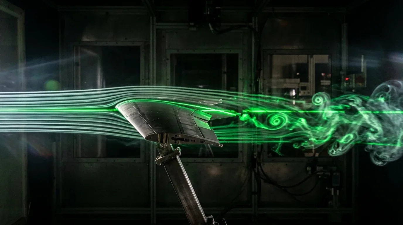
The dissipation Stam accepted smears out exactly the small eddies that make a fluid look alive. The games paper notes that Fedkiw and colleagues proposed vorticity confinement to add back the energy the method loses, encouraging small-scale swirling. The simulator implements it: it computes the curl of the velocity field, ω = ∂v/∂x − ∂u/∂y, takes the normalised gradient of |ω|, which points toward the centre of each vortex, and applies a force along N × ω that spins the existing eddies up. The Vorticity boost slider scales that force. At zero the flow goes soft and laminar within seconds; turned up, a single drag of the mouse breaks into a string of counter-rotating vortices that persist for a long time. Switch to the Vorticity view to see them as red and blue blobs.

Why the GPU

Every cell at once

Each of the four stages is the same small calculation applied to every cell, reading only its neighbours. The simulator runs them as WebGL fragment shaders over a pair of floating-point textures, the same ping-pong arrangement as the reaction–diffusion simulator in this series. The Jacobi relaxation used for the pressure solve is slower to converge than Stam’s Gauss–Seidel but has no dependency between cells, so a single shader pass does one sweep over the whole grid. Twenty-four sweeps a frame, the default, keeps the divergence small enough to be invisible.

A note on what the simulator is not. It is two-dimensional, it has no boundaries other than the edges of the canvas, and the dissipation means the Reynolds number is far lower than anything in a real river. The El Niño article on this site deals with the ocean models that do solve the real equations, on supercomputers, with the opposite trade-off.

Experiments worth running

• Set Viscosity to zero and Vorticity boost high, then draw one slow stroke. Count the vortices it sheds.
• Set Pressure iters to 4 and drag fast. The fluid bunches and stretches in ways no incompressible fluid should; raise the iterations and the artefact disappears.
• Turn Dye fade to zero, switch to Pressure view, and drag in a circle. The pressure field shows the low-pressure core of the vortex and the high-pressure ring where the fluid is being pushed aside.
• Drive Viscosity to maximum. Every stroke dies within a second; this is the honey end of the scale.
• Fire Random splats with Vorticity boost at zero, then again at maximum, and compare how long the motion lasts.

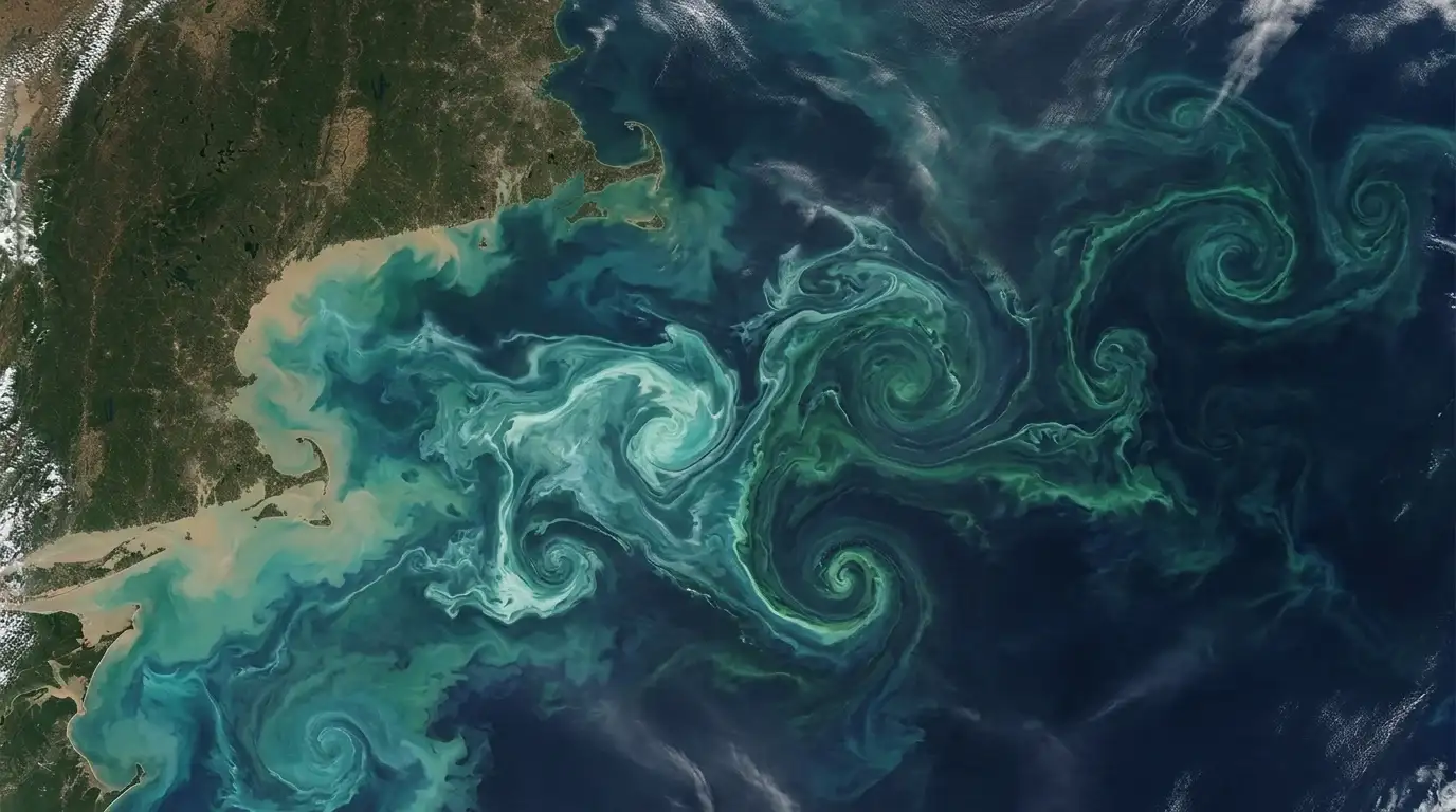
The photographs the simulator is trying to imitate are collected in Milton Van Dyke’s An Album of Fluid Motion, a book of laboratory flow photographs: vortex streets, boundary layers, jets and wakes, the real versions of what the canvas approximates.

Sources

• History, incompressibility, applications: Wikipedia, Navier–Stokes equations
• The Millennium Prize problem, Leray, the 2-D case: Wikipedia, Navier–Stokes existence and smoothness
• OpenAI’s September 2026 claim and the Clay Institute’s response: The Cornell Daily Sun, 9 October 2026
• The method, stability claim, dissipation, projection: Jos Stam, “Stable Fluids” (PDF)
• The 100-line solver, Gauss–Seidel, vorticity confinement: Jos Stam, “Real-Time Fluid Dynamics for Games” (PDF)
• Stam’s Academy Award and Maya Fluid Effects: Wikipedia, Jos Stam
• Video: PapersWeLove, “Stable Fluids” by Dan Piponi
• Book: An Album of Fluid Motion on Amazon (affiliate link)