Double Pendulum Chaos: Watch Two Identical Pendulums Disagree, and Measure How Fast

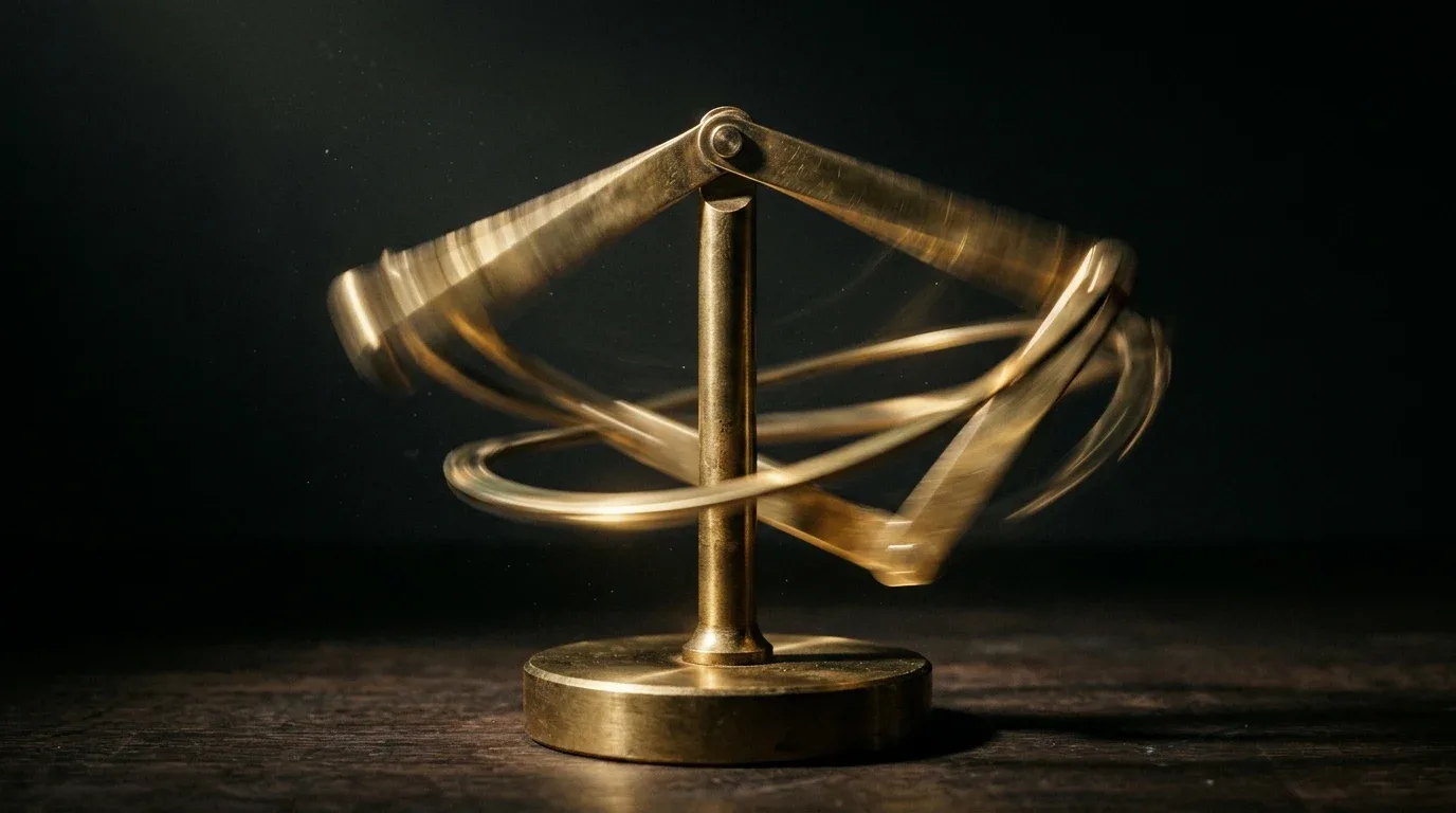
Hang a pendulum from the end of another pendulum and you have built the simplest machine that nobody can predict. A single pendulum is a clock. Attach a second arm to its bob and the motion stays perfectly deterministic, governed by two coupled equations with no randomness anywhere, yet two copies launched a ten-thousandth of a radian apart will be swinging in opposite directions within seconds. The simulator in this article runs two or three such copies side by side and plots the distance between their tips on a logarithmic axis. The line it draws is the signature of chaos, and the slope of that line is a number physicists have a name for.

Video: 2swap, “Double Pendulums are Chaoticn’t”

What the simulator does

Three pendulums, one difference, one graph

Pendulum A starts from whichever preset is selected. Pendulum B starts in the same place except that its upper arm is rotated by Δθ, set on the slider anywhere from a tenth of a radian down to a millionth. Tick “third copy” and pendulum C starts at −Δθ. All of them are integrated with the same fourth-order Runge–Kutta scheme at two thousand steps per simulated second, which is why the energy drift readout in the header sits at zero to four decimal places: the integrator is not the source of the disagreement.

The right-hand panel plots the distance between the tips of A and B against time, on a log scale running from a hundredth of a millimetre up to the full reach of the arms. For the first fraction of a second the two copies are indistinguishable. Then the gap starts to climb, and on a logarithmic axis exponential growth is a straight line. When the line reaches the top, the pendulums have nothing left in common.

Pause the simulation and the bobs can be dragged to any starting position. The mass ratio slider changes the second bob’s weight; air damping adds a drag term; the trace toggle draws the tip paths.

Why a double pendulum is chaotic and a single one is not

Two angles, coupled, and an energy that lets the arms flip

A single pendulum has one angle to track and one conserved energy, and that is enough to pin down its entire future: it swings between the same two turning points forever. The double pendulum has two angles, θ₁ and θ₂, and still only one conserved energy. Newtonian mechanics is cumbersome for it, so physicists write the Lagrangian in terms of the two angles and derive two coupled second-order equations of motion. Those equations are exact. The system can only be solved numerically, and the simulator’s Runge–Kutta loop is that numerical solution, step by step.

Chaos is not guaranteed. At low energy, where neither arm has enough speed to swing over the top, the motion is regular and two nearby starts stay nearby. Load the “Low energy” preset and the divergence graph barely moves. The boundary of that regular region is set by energy conservation: inside it, it is energetically impossible for either pendulum to flip. Outside it, flipping can happen, and whether a given start flips, and when, is where the strong sensitivity to initial conditions takes over. The “High energy” preset starts with both arms raised almost to the vertical, well outside the regular region, which is why its graph climbs from the first second.

The slope of the line

Lyapunov exponents, and reading one off the screen

Suppose two trajectories start a distance d₀ apart and the distance grows as d₀·e^(λt). The constant λ is the Lyapunov exponent. A positive λ means errors grow exponentially and the system is chaotic; zero or negative means they do not. On a log-scale plot of distance against time, λ is the slope. The simulator’s graph does not print the number, but the straight stretch of the red line is λ made visible, and its steepness changes with the starting energy, the mass ratio and the damping. Chaos researchers map Lyapunov exponents against starting angles across the whole range of initial conditions; the simulator samples one such point at a time.

Two consequences follow. First, halving Δθ does not buy twice as long before divergence; it buys one more doubling time, which at high energy is a fraction of a second. Set the slider to a millionth of a radian and the pendulums still part company within the first ten seconds. Second, measurement precision has a hard ceiling. No instrument records an angle to a millionth of a radian, so no real double pendulum’s future beyond a few seconds can be known from its present. The equations are deterministic. The prediction is not.

Where sensitive dependence was discovered

A rounded number in 1961, and a butterfly in 1972

The idea predates the pendulum demonstration. Henri Poincaré, working on the three-body problem in 1890, found that small differences in initial conditions could produce large differences in outcome, and suggested the same could hold in meteorology. The modern form arrived at MIT. Edward Lorenz, a research scientist in the Department of Meteorology, was running a weather model in 1961 on a Royal McBee LGP-30 and wanted to repeat a run from the middle. He typed in the values from the printout. The machine stored six digits, but the printout showed three: a value like 0.506127 printed as 0.506. The rerun diverged from the original until the two forecasts shared nothing.

Lorenz published the theory in 1963 as “Deterministic Nonperiodic Flow” in the Journal of the Atmospheric Sciences. The nickname came later: for a 1972 talk at the American Association for the Advancement of Science, the meteorologist Philip Merilees proposed the title “Does the flap of a butterfly’s wings in Brazil set off a tornado in Texas?”, and “the butterfly effect” has been the public name for sensitive dependence ever since. The double pendulum is the same phenomenon with the atmosphere replaced by two sticks and a hinge, which is why it has become the standard tabletop demonstration.

Where the double pendulum turns up outside the classroom

Skyscrapers and the absence of a natural frequency

A single pendulum has a resonant frequency, and anything driven at that frequency will swing harder and harder. A double pendulum has none, because its motion never settles into one period. That absence is useful. The lack of a natural excitation frequency has led to double pendulum systems in seismic resistance designs: the building is the primary inverted pendulum and a secondary mass completes the system, so that an earthquake’s shaking has no single frequency to lock onto. The chaos that makes the toy unpredictable is what makes the structure hard to resonate.

Experiments worth running

• Load “High energy” with the third copy on and Δθ at 1e-4. Count the seconds until A, B and C are visibly doing three different things. Then set Δθ to 1e-6 and count again. The second number is only slightly larger.
• Switch to “Low energy.” The graph flattens. Nudge the bobs upward while paused, reset, and find the energy at which the straight line first appears.
• Turn on air damping with the high-energy start. Divergence still happens, but the exponent falls as energy drains and the system eventually becomes regular.
• Drag the mass ratio to 3. The light upper bob gets whipped by the heavy lower one and the tip traces change character entirely.

The simulator is a single page at apps.x9m8.com/double-pendulum with the source on GitHub. For the gravitational version of the same lesson, three bodies instead of two arms, see Gravity Lab and its article. The popular history of all of this is James Gleick’s Chaos: Making a New Science, which tells the Lorenz story in full.

Sources

• Double pendulum mechanics, numerical solution, flipping threshold, Lyapunov maps and seismic use: Wikipedia, Double pendulum
• Lorenz’s 1961 rounding incident, MIT career and the 1963 paper: Wikipedia, Edward Norton Lorenz
• Poincaré, the 1972 talk title and the term “sensitive dependence on initial conditions”: Wikipedia, Butterfly effect
• Video: 2swap, Double Pendulums are Chaoticn’t
• Book: Chaos: Making a New Science on Amazon (affiliate link)