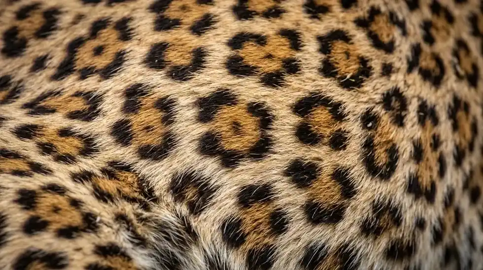
Two chemicals, one grid, two numbers to tune. That is the full ingredient list for the simulation in this article, and it produces leopard spots, zebra stripes, coral branches, dividing cells and worm-like labyrinths depending on where the two numbers sit. Alan Turing wrote down the general idea in 1952 while trying to explain how an embryo, which starts as a sphere with no front or back, ends up with a pattern. He had no computer fast enough to run it. A browser with WebGL runs it at hundreds of thousands of cells, ten times a frame.
Video: MinuteEarth, “Can Math Explain How Animals Get Their Patterns?”
What the simulator does
Eight presets, two sliders, and a brush
The canvas holds a field of two chemicals, A and B, rendered as a colour map. The Pattern menu picks from eight named regions of the parameter space: Coral, Mitosis, Spots, Stripes, Moving spots, Holes, Chaos and Solitons. Custom unlocks the two sliders, feed f and kill k, so the parameters can be dragged continuously from one regime into another and the pattern reorganises itself on the way. Palette changes the colour mapping. The mouse paints chemical B onto the grid, which is how patterns are seeded; Clear wipes the field, Reset reseeds it, and the step counter in the header shows how many iterations have run.
Every frame the simulator runs ten update passes on the GPU, so the step counter climbs by ten per frame. The whole thing is one HTML file at apps.x9m8.com/reaction-diffusion, with the source on GitHub.
What a reaction–diffusion system is
Reactions that change chemicals, diffusion that spreads them
The term describes a family of models in which chemical concentrations change through local reactions that transform the substances into each other, combined with diffusion that spreads them across space. Mathematically they are semi-linear parabolic partial differential equations: one equation per chemical, each with a diffusion term and a reaction term. Applications run well beyond chemistry: morphogenesis, animal coats, ecological invasions, the spread of epidemics, tumour growth, wound healing, plasma physics, even models of visual hallucination.
The particular model in the simulator is Gray–Scott. Chemical A is fed into the grid at a rate f, chemical B is removed at a rate f + k, and the reaction A + 2B → 3B converts A into B wherever B is already present. Written out:
- ∂A/∂t = D_A ∇²A − A·B² + f (1 − A)
- ∂B/∂t = D_B ∇²B + A·B² − (f + k) B
Karl Sims’s reaction–diffusion tutorial, which this implementation follows, uses diffusion rates D_A = 1.0 and D_B = 0.5, so, in his words, “A diffuses faster than B.” The Laplacian ∇² is approximated on the grid by a 3×3 convolution with a centre weight of −1, 0.2 on the four edge neighbours and 0.05 on the four corners. Sims gives f = 0.0367, k = 0.0649 for mitosis, where a spot of B grows and then divides in two like a cell, and f = 0.0545, k = 0.062 for coral growth. Those are the simulator’s Mitosis and Coral presets.
The other presets sit at nearby points on the same map. Spots run at f = 0.030, k = 0.062; Stripes, labelled worms in the menu, at f = 0.025, k = 0.060; Moving spots at f = 0.014, k = 0.054; Holes at f = 0.078, k = 0.061; Chaos at f = 0.022, k = 0.051; and Solitons, isolated blobs that hold their shape, at f = 0.062, k = 0.0609. The feed slider runs from 0.005 to 0.10 and the kill slider from 0.040 to 0.075, which covers every regime in the list with room on either side to watch a pattern die.
The reason the patterns are so sensitive is that only a thin band of the (f, k) plane produces anything at all. Too much kill and B dies out everywhere, leaving uniform A. Too little and B takes over everywhere. The spots, stripes and labyrinths live on the boundary between those two fates, which is why dragging the sliders a few thousandths in either direction changes everything.
Turing’s paper
A sphere with no front, and chemicals that break the symmetry
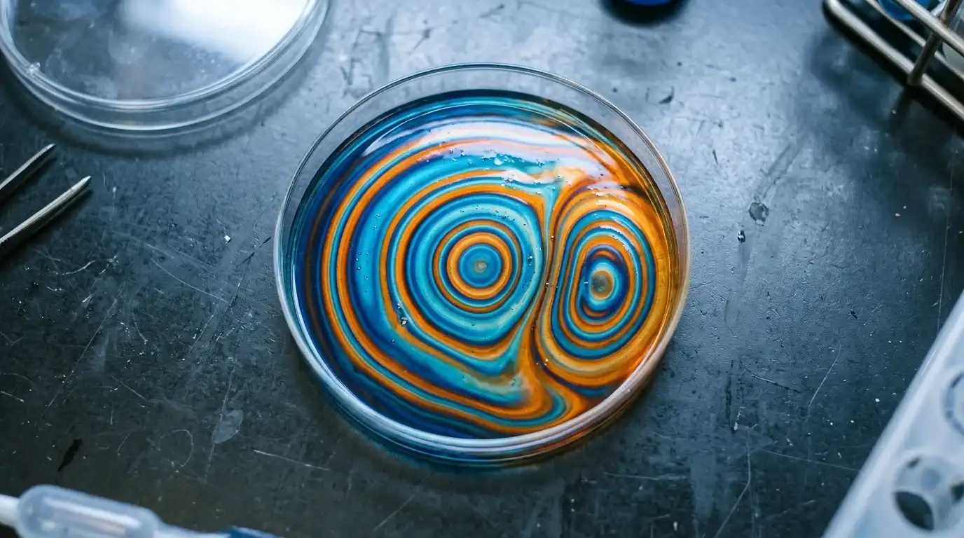
Turing turned to biology in 1951, at 39, and in January 1952 published “The Chemical Basis of Morphogenesis” in the Philosophical Transactions of the Royal Society of London B. His question, as the Wikipedia account of Turing patterns puts it, was “how is spatial information generated in organisms?” His answer was that chemicals reacting with each other and diffusing across space could account for the main phenomena of morphogenesis. The key finding was that patterns form when an activator also produces an inhibitor, and the two diffuse at different rates.
The counterintuitive part is that diffusion, which usually smooths things out, is what creates the pattern. A reaction that is stable on its own, settling to a uniform grey, can become unstable once diffusion is added, because a state that is stable in the local system can become unstable in the presence of diffusion. Turing’s model amplifies some wavelengths and suppresses others, and the surviving wavelength sets the spacing of the spots or stripes.
Computers were scarce in 1951, so Turing solved linear approximations by hand. The paper predates the discovery of DNA’s structure and is still considered seminal in mathematical biology. Boris Belousov observed a real chemical oscillator around the same period, could not get it published, and was unaware of Turing’s work; the Belousov–Zhabotinsky reaction is now a standard example of a reaction–diffusion system with more than two components.
Where the patterns turn up in living things
Fish, feathers, fingers and chia seeds
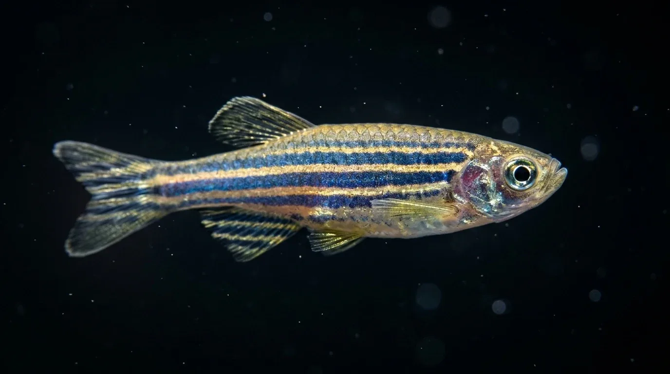
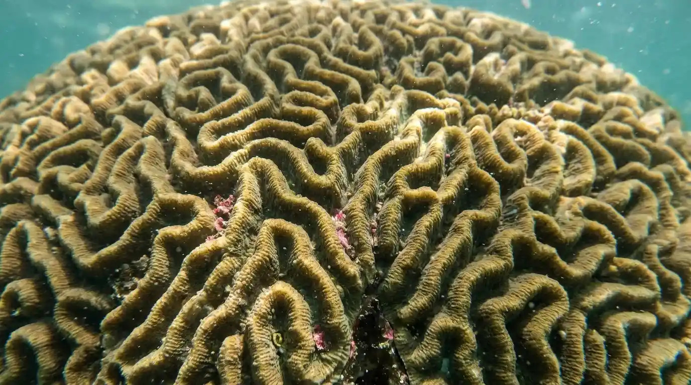
The biological evidence took decades. James Murray used Turing’s paper to explain the spots and stripes on cat fur. Later work suggests the mechanism partly explains feathers, hair follicles, lung branching and left-right asymmetry. The Turing pattern article lists zebrafish pigmentation, where the patterns arise from interactions between pigment cells, along with chick feather patterns, the cusps on mouse and vole teeth, and mouse hair-follicle precursors that form by self-aggregation without any pre-pattern telling them where to go.
Two results are worth singling out. In 2012, Sheth and colleagues removed Hox genes in mice and found the number of digits went up without the limb getting larger, which suggests the genes tune the wavelength of a Turing-type mechanism rather than specifying each finger. And in 2023 a study presented through the American Physical Society grew chia seeds in trays with adjusted moisture; patterns resembling natural ones emerged, which is believed to be the first experimental verification of Turing’s insight using living vegetation. The Mitosis preset in the simulator is the closest thing to watching the mechanism at work: a single blob of B that cannot stay a blob.
Why it runs on the GPU
Ping-pong textures and a fragment shader
A reaction–diffusion step is the same small calculation applied to every cell, with each cell reading only its eight neighbours. That is exactly the shape of work a graphics card is built for. The simulator stores A and B in a floating-point texture, and a fragment shader computes the Laplacian, the reaction and the feed and kill terms for every pixel at once, writing the result into a second texture. The two textures then swap roles, the classic ping-pong arrangement, and the shader runs again. Ten passes per frame at sixty frames a second is six hundred iterations a second across the whole grid, which is why a coral preset fills the screen in a few seconds rather than a few minutes.
The same approach drives the fluid simulator in this series. For the opposite extreme, patterns that come from discrete rules rather than continuous chemistry, the cellular automata article covers Conway’s Life and Wolfram’s elementary rules.
Experiments worth running
- Load Coral, let it fill half the screen, then switch to Custom and nudge k up by 0.002 at a time. Find the value where growth stops and the coral begins to dissolve.
- Load Spots, then slowly lower f. The spots start to stretch and join into stripes, the same transition that separates a leopard from a zebra in the biological models.
- Load Mitosis and paint a single dot. Count the divisions before the dots fill the field.
- Load Solitons and paint two dots close together. Watch whether they merge, repel or annihilate.
- Pick Chaos and leave it running. The pattern never settles, which is the regime where the simple system behaves least like a crystal and most like weather.
Philip Ball’s Patterns in Nature collects the spots, stripes, branches and spirals that this mechanism and a handful of others produce, with the photographs the simulator is trying to imitate.
Patterns in Nature: Why the Natural World Looks the Way It Does by Philip Ball. Spots, stripes, branches, spirals and the handful of mechanisms behind them, with the photographs. See it on Amazon (affiliate link)
As an Amazon Associate I earn from qualifying purchases. A commission may be earned if you buy through this link, at no extra cost to you.
Sources
- Turing’s 1952 paper, hand-solved approximations, Murray’s cat-fur work, the 2012 Hox result and the 2023 chia study: Wikipedia, Alan Turing
- Activator–inhibitor mechanism, biological examples, Turing’s question: Wikipedia, Turing pattern
- Definition, instability with diffusion, applications, Belousov–Zhabotinsky: Wikipedia, Reaction–diffusion system
- Gray–Scott parameters, Laplacian weights, diffusion rates, mitosis and coral values: Karl Sims, Reaction-Diffusion Tutorial
- Video: MinuteEarth, Can Math Explain How Animals Get Their Patterns?
- Book: Patterns in Nature on Amazon (affiliate link)